Clustering

Clustering is implemented in two classes, HCA and K-Means. Using classes for clustering simplifies explorative analysis as for example different visualisations can be generated without recalculating the clusters.

Hierarchical cluster analysis

class autoprot.analysis.clustering.HCA(*args, **kwargs)

Conduct hierarchical cluster analysis.

Notes

User provides dataframe and can afterwards use various metrics and methods to perfom and evaluate clustering.

StandarWorkflow: makeLinkage() -> findNClusters() -> makeCluster()

Examples

First grab a dataset that will be used for clustering such as the iris dataset. Extract the species labelling from the dataframe as it cannot be used for clustering and will be used later to evaluate the result.

Initialise the clustering class with the data and find the optimum number of clusters and generate the final clustering with the autoRun method.

df = sns.load_dataset('iris')
labels = df.pop('species')
c = ana.HCA(df)
c.auto_run()

(Source code, png, hires.png, pdf)

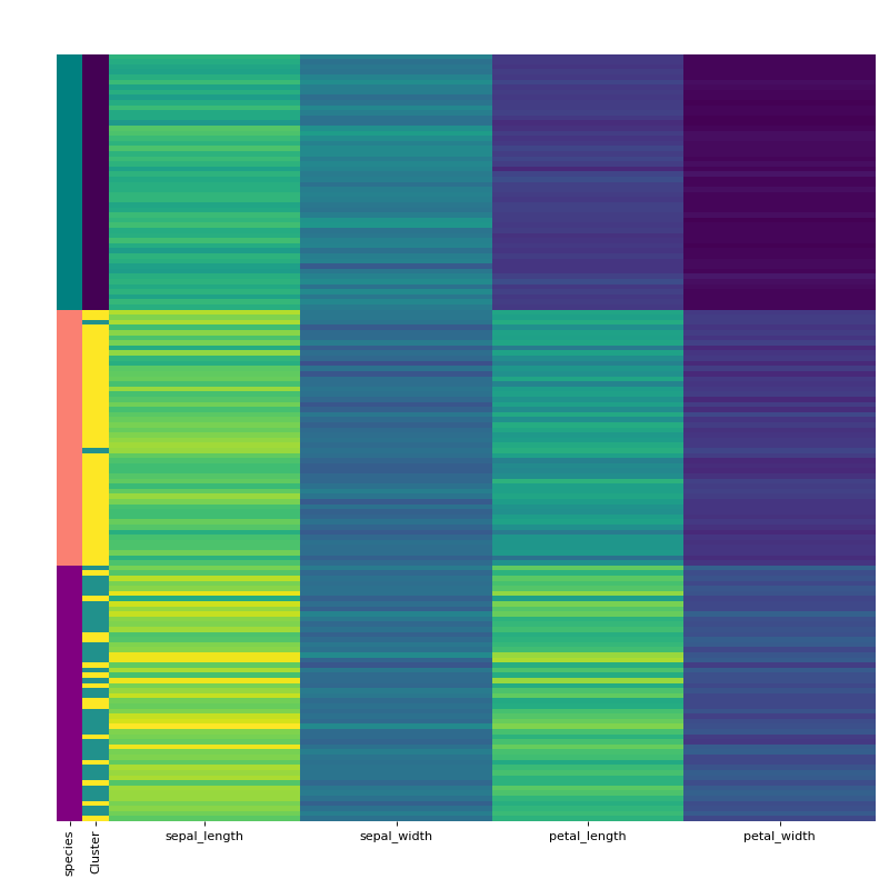
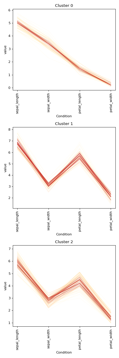
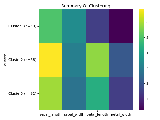
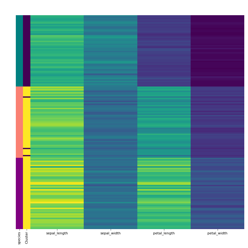
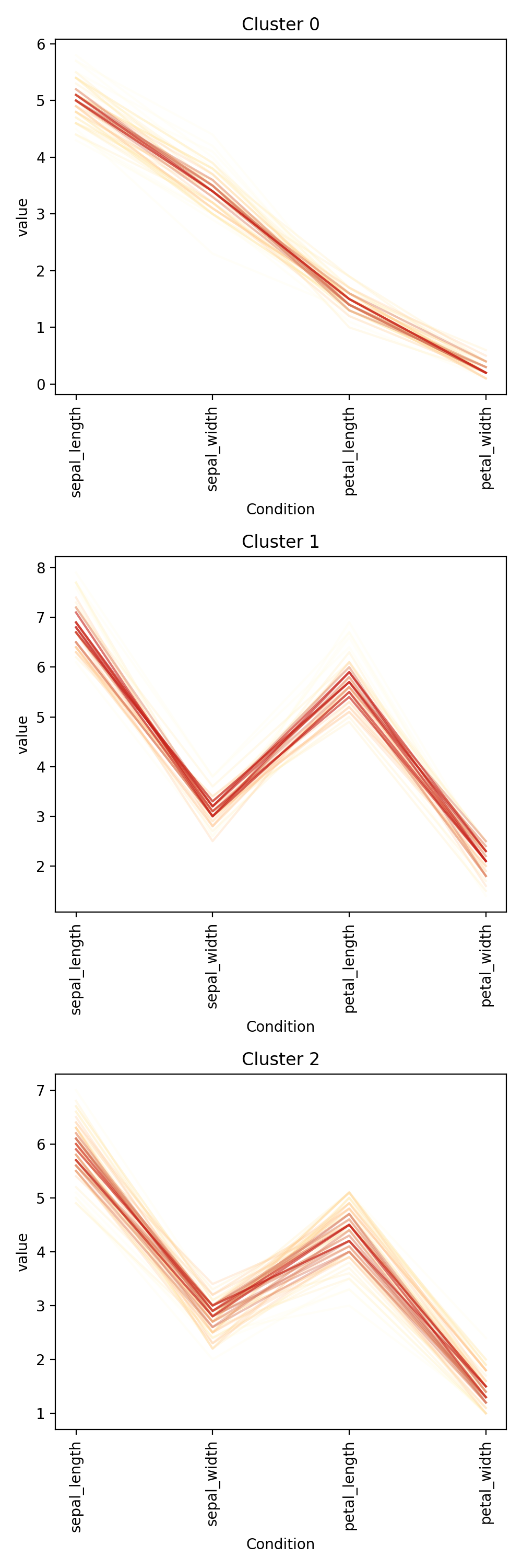
Finally, visualise the clustering using the vis_cluster method and include the previously extracted labeling column from the original dataframe.

labels.replace(['setosa', 'virginica', 'versicolor'], ["teal", "purple", "salmon"], inplace=True)
rc = {"species" : labels}
c.vis_cluster(row_colors={'species': labels})

(Source code, png, hires.png, pdf)

HCA separates the setosa quite well but virginica and versicolor are harder. When we manually pick true the number of clusters, HCA performs only slightly better von this dataset. Note that you can change the default cmap for the class by changing the cmap attribute.

c.nclusters = 3
c.make_cluster()
c.cmap = 'coolwarm'
c.vis_cluster(row_colors={'species': labels}, make_traces=True, file=None, make_heatmap=True)

(Source code)

(png, hires.png, pdf)

(png, hires.png, pdf)

(png, hires.png, pdf)

auto_run(start_processing=1, stop_processing=5)

Automatically run the clustering pipeline with standard settings.

Parameters:

• start_processing (int, optional) – Step of the pipeline to start. The default is 1.

• stop_processing (int, optional) – Step of the pipeline to stop. The default is 5.

Notes

The pipeline currently consists of (1) makeLinkage, (2) findNClusters and (3) makeCluster.

Return type:

None.

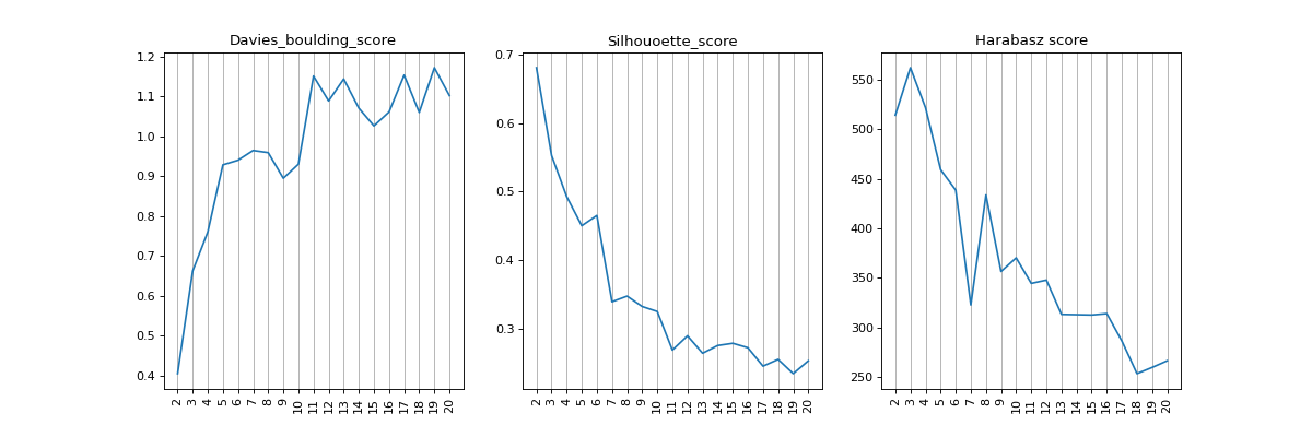
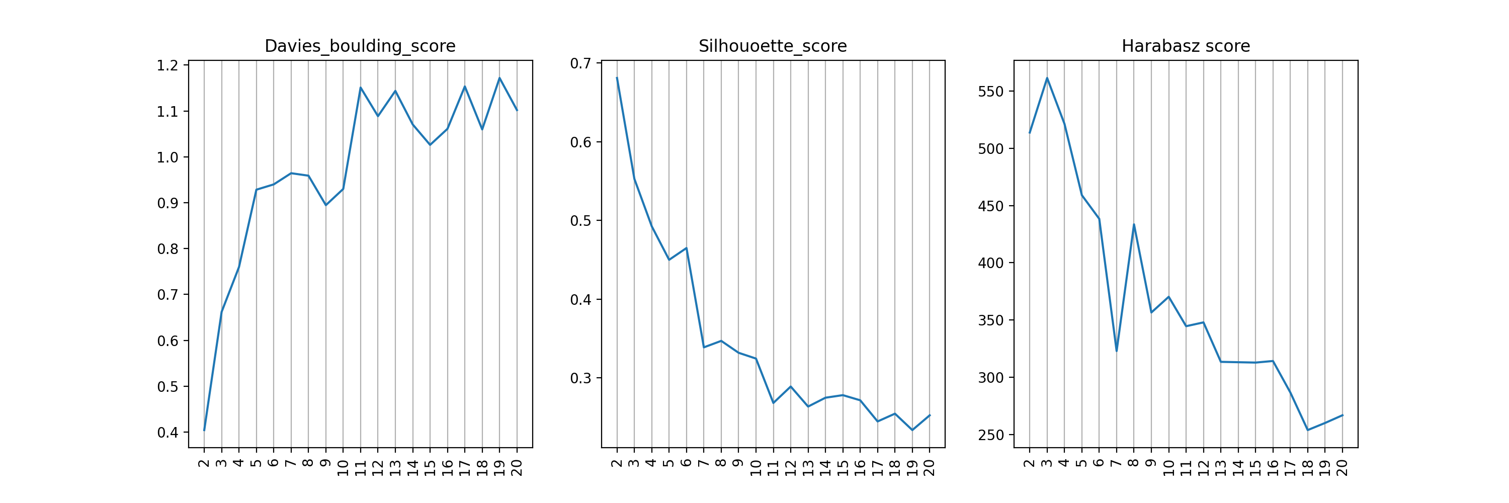
find_nclusters(start=2, up_to=20, figsize=(15, 5), plot=True)

Evaluate number of clusters.

Parameters:

• start (int, optional) – The minimum number of clusters to plot. The default is 2.

• up_to (int, optional) – The maximum number of clusters to plot. The default is 20.

• figsize (tuple of float or int, optional) – The size of the plotted figure. The default is (15,5).

• plot (bool, optional) – Whether to plot the corresponding figures for the cluster scores

Notes

Davies-Bouldin score:

The score is defined as the average similarity measure of each cluster with its most similar cluster, where similarity is the ratio of within-cluster distances to between-cluster distances. Thus, clusters which are farther apart and less dispersed will result in a better score. The minimum score is zero, with lower values indicating better clustering.

Silhouette score:

The Silhouette Coefficient is calculated using the mean intra-cluster distance (a) and the mean nearest-cluster distance (b) for each sample. The Silhouette Coefficient for a sample is (b - a) / max(a, b). To clarify, b is the distance between a sample and the nearest cluster that the sample is not a part of. Note that Silhouette Coefficient is only defined if number of labels is 2 <= n_labels <= n_samples - 1. The best value is 1 and the worst value is -1. Values near 0 indicate overlapping clusters. Negative values generally indicate that a sample has been assigned to the wrong cluster, as a different cluster is more similar.

Harabasz score:

It is also known as the Variance Ratio Criterion. The score is defined as ratio between the within-cluster dispersion and the between-cluster dispersion.

Return type:

None.

make_cluster()

Form flat clusters from the hierarchical clustering of linkage.

Return type:

None.

make_linkage(method='single', metric: Literal['braycurtis', 'canberra', 'chebyshev', 'cityblock', 'correlation', 'cosine', 'dice', 'euclidean', 'hamming', 'jaccard', 'jensenshannon', 'kulczynski1', 'mahalanobis', 'matching', 'minkowski', 'rogerstanimoto', 'russellrao', 'seuclidean', 'sokalmichener', 'sokalsneath', 'sqeuclidean', 'yule', 'spearman', 'pearson'] = 'euclidean')

Perform hierarchical clustering on the data.

Parameters:

• method (str) – Which method is used for the clustering. Possible are ‘single’, ‘average’ and ‘complete’ and all values for method of scipy.cluster.hierarchy.linkage See: https://docs.scipy.org/doc/scipy/reference/generated/scipy.cluster.hierarchy.linkage.html

• metric (str or function) – Which metric is used to calculate distance. Possible values are ‘pearson’, ‘spearman’ and all metrics implemented in scipy.spatial.distance.pdist See: https://docs.scipy.org/doc/scipy/reference/generated/scipy.spatial.distance.pdist.html

Return type:

None.

K-Means clustering

class autoprot.analysis.clustering.KMeans(*args, **kwargs)

Perform KMeans clustering on a dataset.

Return type:

None.

Notes

The functions uses scipy.cluster.vq.kmeans2 (see https://docs.scipy.org/doc/scipy/reference/generated/scipy.cluster.vq.kmeans2.html#scipy.cluster.vq.kmeans2)

References

D. Arthur and S. Vassilvitskii, “k-means++: the advantages of careful seeding”, Proceedings of the Eighteenth Annual ACM-SIAM Symposium on Discrete Algorithms, 2007.

Examples

First grab a dataset that will be used for clustering such as the iris dataset. Extract the species labelling from the dataframe as it cannot be used for clustering and will be used later to evaluate the result.

Initialise the clustering class with the data and find the optimum number of clusters and generate the final clustering with the autoRun method.

df = sns.load_dataset('iris')
labels = df.pop('species')
c = ana.KMeans(df)
c.auto_run()

(Source code, png, hires.png, pdf)

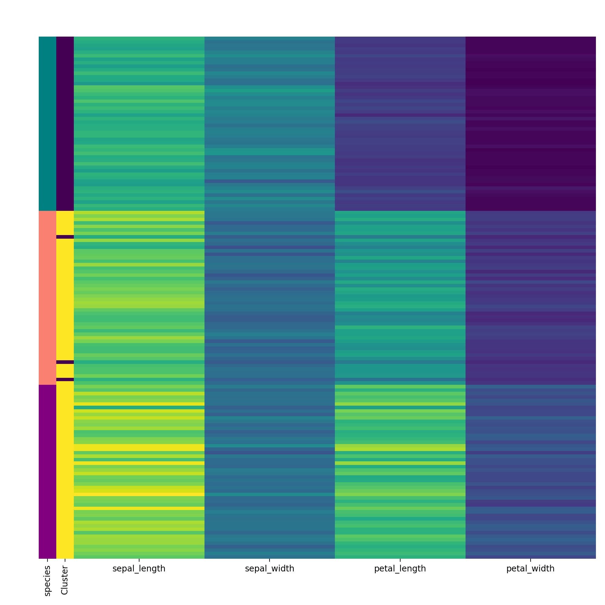
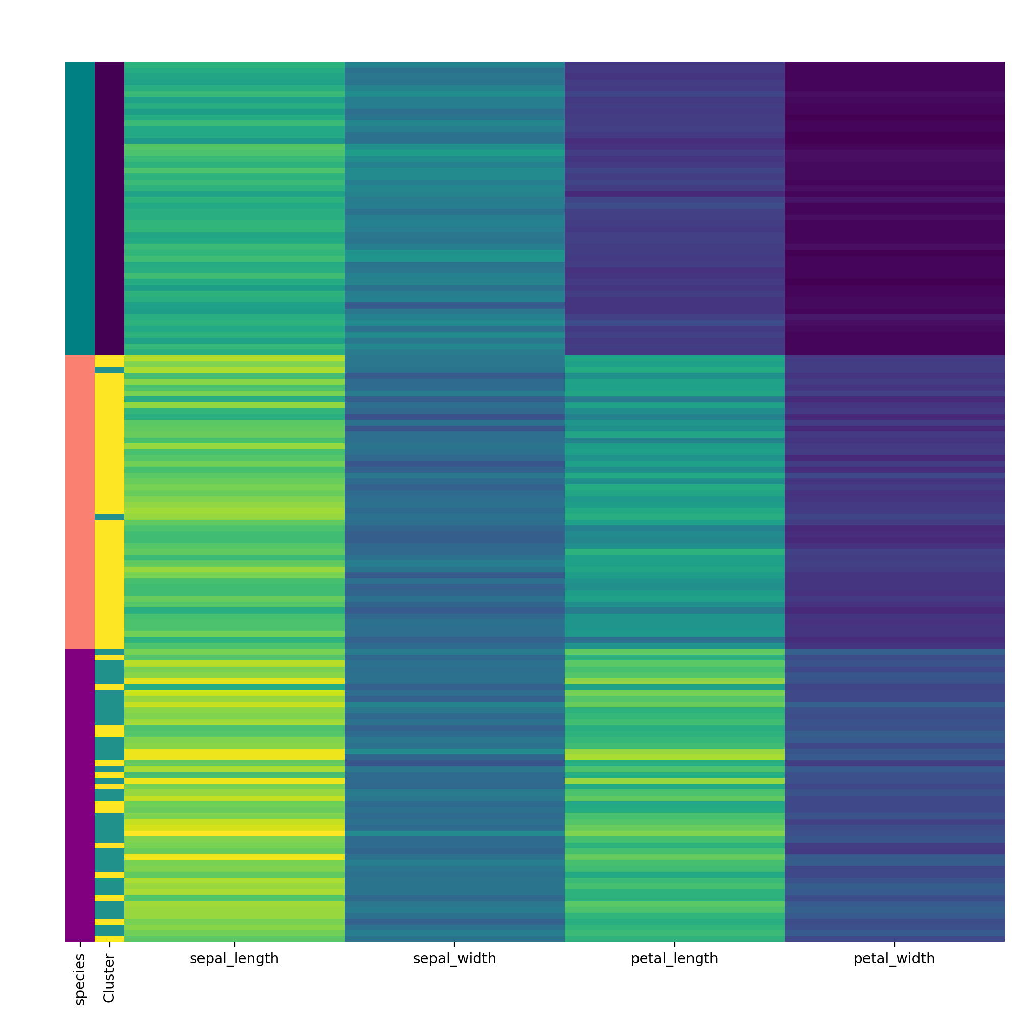
Finally, visualise the clustering using the visCluster method and include the previously extracted labeling column from the original dataframe.

labels.replace(['setosa', 'virginica', 'versicolor'], ["teal", "purple", "salmon"], inplace=True)
rc = {"species" : labels}
c.vis_cluster(row_colors={'species': labels})

(Source code, png, hires.png, pdf)

As you can see can KMeans quite well separate setosa but virginica and versicolor are harder. When we manually pick the number of clusters, it gets a bit better

c.nclusters = 3
c.make_cluster()
c.vis_cluster(row_colors={'species': labels}, make_traces=True, file=None, make_heatmap=True)

(Source code)

(png, hires.png, pdf)

(png, hires.png, pdf)

(png, hires.png, pdf)

auto_run(start_processing=1, stop_processing=5)

Automatically run the clustering pipeline with standard settings.

Parameters:

• start_processing (int, optional) – Step of the pipeline to start. The default is 1.

• stop_processing (int, optional) – Step of the pipeline to stop. The default is 5.

Notes

The pipeline currently consists of (1) findNClusters and (2) makeCluster.

Return type:

None.

find_nclusters(start=2, up_to=20, figsize=(15, 5), plot=True, algo='scipy')

Evaluate number of clusters.

Parameters:

• start (int, optional) – The minimum number of clusters to plot. The default is 2.

• up_to (int, optional) – The maximum number of clusters to plot. The default is 20.

• figsize (tuple of float or int, optional) – The size of the plotted figure. The default is (15,5).

• plot (bool, optional) – Whether to plot the corresponding figures for the cluster scores

• algo (str, optional) – Algorith to use for KMeans Clustering. Either “scipy” or “sklearn”

Notes

Davies-Bouldin score:

The score is defined as the average similarity measure of each cluster with its most similar cluster, where similarity is the ratio of within-cluster distances to between-cluster distances. Thus, clusters which are farther apart and less dispersed will result in a better score. The minimum score is zero, with lower values indicating better clustering.

Silhouette score:

The Silhouette Coefficient is calculated using the mean intra-cluster distance (a) and the mean nearest-cluster distance (b) for each sample. The Silhouette Coefficient for a sample is (b - a) / max(a, b). To clarify, b is the distance between a sample and the nearest cluster that the sample is not a part of. Note that Silhouette Coefficient is only defined if number of labels is 2 <= n_labels <= n_samples - 1. The best value is 1 and the worst value is -1. Values near 0 indicate overlapping clusters. Negative values generally indicate that a sample has been assigned to the wrong cluster, as a different cluster is more similar.

Harabasz score:

It is also known as the Variance Ratio Criterion. The score is defined as ratio between the within-cluster dispersion and the between-cluster dispersion.

Return type:

None.

make_cluster(algo='scipy', **kwargs)

Perform k-means clustering and store the resulting labels in self.clusterId.

Parameters:

• algo (str, optional) – Algorith to use for KMeans Clustering. Either “scipy” or “sklearn”

• **kwargs – passed to either scipy or sklearn kmeans

Return type:

None.