Various Statistical Tools#
Autoprot Analysis Functions.
@author: Wignand, Julian, Johannes
@documentation: Julian
- autoprot.analysis.stats.edm(matrix_a, matrix_b)[source]#
Calculate an euclidean distance matrix between two matrices.
See: https://medium.com/swlh/euclidean-distance-matrix-4c3e1378d87f
- Parameters:
matrix_a (np.ndarray) – Matrix 1.
matrix_b (np.ndarray) – Matrix 2.
- Returns:
Distance matrix.
- Return type:
np.ndarray
- autoprot.analysis.stats.loess(data, xvals, yvals, alpha, poly_degree=2)[source]#
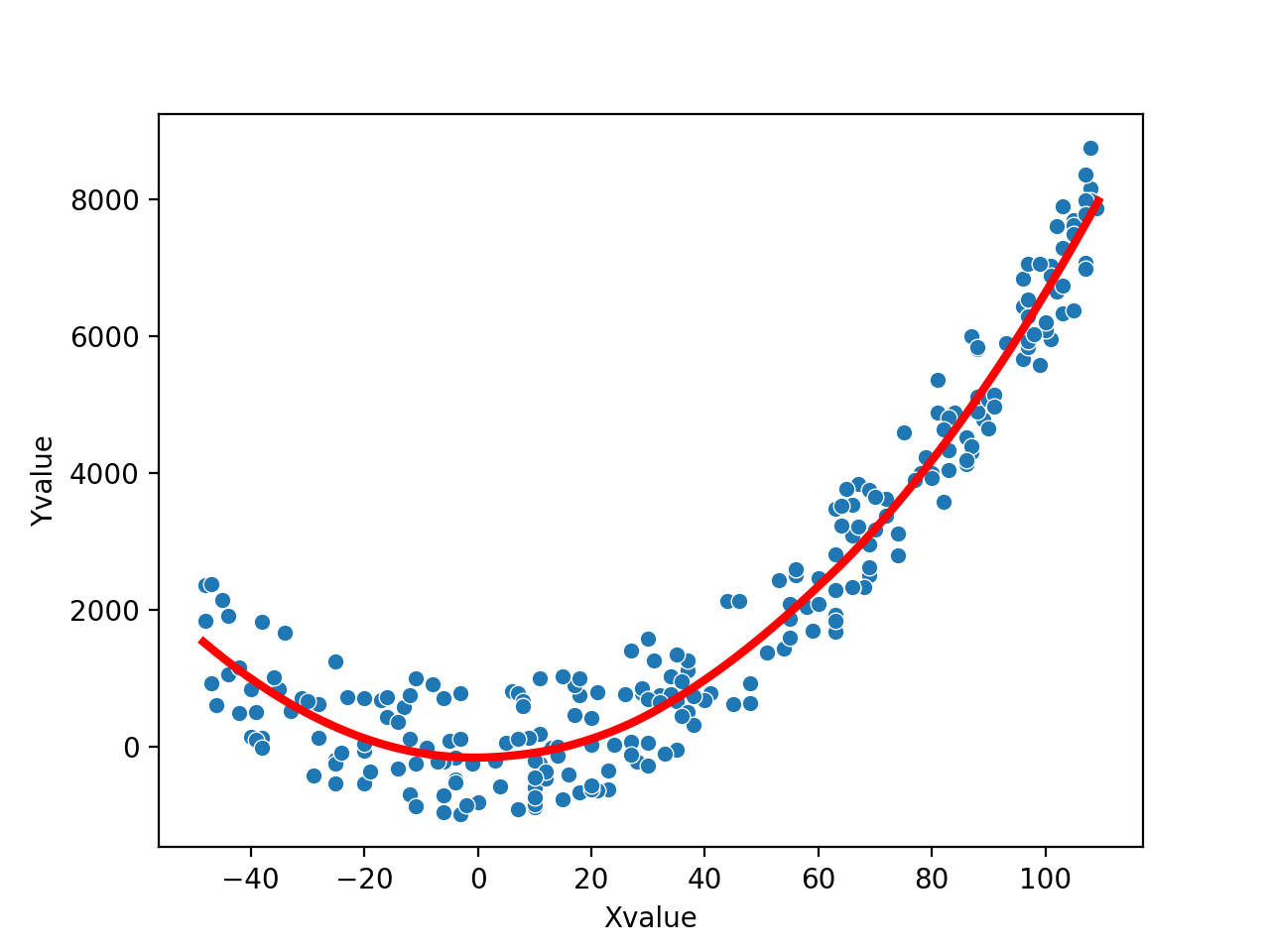
Calculate a LOcally-Weighted Scatterplot Smoothing Fit.
See: https://medium.com/@langen.mu/creating-powerfull-lowess-graphs-in-python-e0ea7a30b17a
- Parameters:
data (pd.Dataframe) – Input dataframe.
xvals (str) – Colname of x values.
yvals (str) – Colname of y values.
alpha (float) – Sensitivity of the estimation. Controls how much of the total number of values is used during weighing. 0 <= alpha <= 1.
poly_degree (int, optional) – Degree of the fitted polynomial. The default is 2.
- Return type:
None.
Notes
Loess normalisation (also referred to as Savitzky-Golay filter) locally approximates the data around every point using low-order functions and giving less weight to distant data points.
Examples
>>> np.random.seed(10)
>>> x_values = np.random.randint(-50,110,size=250)
>>> y_values = np.square(x_values)/1.5 + np.random.randint(-1000,1000, size=len(x_values))
>>> df = pd.DataFrame({"Xvalue" : x_values,
                       "Yvalue" : y_values
                       })
>>> evalDF = autoprot.analysis.loess(df, "Xvalue", "Yvalue", alpha=0.7, poly_degree=2)
>>> fig, ax = plt.subplots(1,1)
>>> sns.scatterplot(df["Xvalue"], df["Yvalue"], ax=ax)
>>> ax.plot(eval_df['v'], eval_df['g'], color='red', linewidth= 3, label="Test")
import autoprot.analysis as ana
import seaborn as sns

x_values = np.random.randint(-50,110,size=(250))
y_values = np.square(x_values)/1.5 + np.random.randint(-1000,1000, size=len(x_values))
df = pd.DataFrame({"Xvalue" : x_values,
                   "Yvalue" : y_values
                   })
evalDF = ana.loess(df, "Xvalue", "Yvalue", alpha=0.7, poly_degree=2)
fig, ax = plt.subplots(1,1)
sns.scatterplot(x=df["Xvalue"], y=df["Yvalue"], ax=ax)
ax.plot(evalDF['v'], evalDF['g'], color='red', linewidth= 3, label="Test")
plt.show()
(
Source code,png,hires.png,pdf)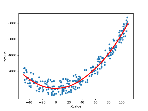
- autoprot.analysis.stats.make_psm(seq, seq_len)[source]#
Generate a position score matrix for a set of sequences.
Returns the percentage of each amino acid for each position that can be further normalized using a PSM of unrelated/background sequences.
- Parameters:
seq (list of str) – list of sequences.
seq_len (int) – Length of the peptide sequences. Must match to the list provided.
- Returns:
Dataframe holding the prevalence for every amino acid per position in the input sequences.
- Return type:
pd.Dataframe
Examples
>>> autoprot.analysis.make_psm(['PEPTIDE', 'PEGTIDE', 'GGGGGGG'], 7)
          0         1         2         3         4         5         6
G  0.333333  0.333333  0.666667  0.333333  0.333333  0.333333  0.333333
P  0.666667  0.000000  0.333333  0.000000  0.000000  0.000000  0.000000
matrix_a  0.000000  0.000000  0.000000  0.000000  0.000000  0.000000  0.000000
V  0.000000  0.000000  0.000000  0.000000  0.000000  0.000000  0.000000
L  0.000000  0.000000  0.000000  0.000000  0.000000  0.000000  0.000000
I  0.000000  0.000000  0.000000  0.000000  0.666667  0.000000  0.000000
M  0.000000  0.000000  0.000000  0.000000  0.000000  0.000000  0.000000
C  0.000000  0.000000  0.000000  0.000000  0.000000  0.000000  0.000000
F  0.000000  0.000000  0.000000  0.000000  0.000000  0.000000  0.000000
Y  0.000000  0.000000  0.000000  0.000000  0.000000  0.000000  0.000000
W  0.000000  0.000000  0.000000  0.000000  0.000000  0.000000  0.000000
H  0.000000  0.000000  0.000000  0.000000  0.000000  0.000000  0.000000
K  0.000000  0.000000  0.000000  0.000000  0.000000  0.000000  0.000000
R  0.000000  0.000000  0.000000  0.000000  0.000000  0.000000  0.000000
Q  0.000000  0.000000  0.000000  0.000000  0.000000  0.000000  0.000000
N  0.000000  0.000000  0.000000  0.000000  0.000000  0.000000  0.000000
E  0.000000  0.666667  0.000000  0.000000  0.000000  0.000000  0.666667
D  0.000000  0.000000  0.000000  0.000000  0.000000  0.666667  0.000000
S  0.000000  0.000000  0.000000  0.000000  0.000000  0.000000  0.000000
T  0.000000  0.000000  0.000000  0.666667  0.000000  0.000000  0.000000